Storage Capacity of a Single Macrocolumn
This page has my original 1996 thesis results characterizing the storage capacity of a single macrocolumn, or "mac". An analysis of the storage capacity of an overall hierarchy of macs is a future project, but this page has my general argument that for naturalistic input domains, such a hierarchical system could operate indefinitely storing all novel, important inputs, and with high likelihood, never reaching capacity.
A Sparsey mac is a set of Q minicolumns each with K units. The minicolumns are WTA competitive modules and abbreviated, "CM". The K units are proposed as analogous to the L2/3 pyramidal population of a real cortical minicolumn. We plan to gradually enrich the model and its correspondence to the other parts of a minicolumn, e.g., the sub-populations in other layers, over time, but we consider the L2/3 population in particular to be the principal repository of memory, most importantly, because it is the largest sub-population of the minicolumn (and thus of the mac, and of the cortical region, and of the whole cortex) and therefore corresponds to the largest possible capacity given our coding scheme. Figure 1a shows a biologically realistically-sized mac (Q=100, K=40) (red outline) (actually, Q=70, K=20 is slightly more realistic).
These experiments use a slightly different architecture than the current model (which is used in all other pages on this site). In the current model: a) all units in a mac's receptive field (RF) connect to all cells in the mac; and b) all codes that ever become active in a mac consist of one winner in each of its Q CMs. Thus, all codes stored in said mac are of the same fixed size, Q. In the model shown in Figure 1a:
- Each individual input feature in the mac's RF (here, the RF is just called the "input level") projects only to the units of its associated CM (gray bundles), i.e., there is a 1-to-1 association of input features to CMs (so in Figure 1, there are only 100x40=4000 bottom-up weights)
- A code will consist of one winner in each CM whose corresponding input feature is active. As shown in Figure 1b, in these studies, each individual input (a frame of a sequence) has only 20 (out of 100) features active. Thus, all codes activated (and thus, stored) consist of 20 active units, one in each of the 20 CMs whose corresponding input feature is active on that frame.
Note that although the bottom-up (U) connectivity scheme of the model of Figure 1a differs from that of the current version of the model, the horizontal connectivity scheme is the same, i.e., all mac units project to all other mac units except those in the source unit's CM. Thus, in the depicted model, there are 4000 x 3960 = 15,840,000 H weights (a tiny sample of which suggested by the green arrow sprays). Figure 1b shows the nature of the random sequences used in these studies. Each input sequence has 10 frames and 20 out of 100 features are chosen randomly to be active on each frame.
Despite this variant architecture, we believe these capacity results would be qualitatively similar to those that would result for the general architecture case (i.e., full connectivity from input units to all of the mac's units, as seen on this site's other pages), that is, the number of inputs that can be stored increases faster-than-linearly in the units and linearly in the weights. Studies confirming this are on the list for near future projects.
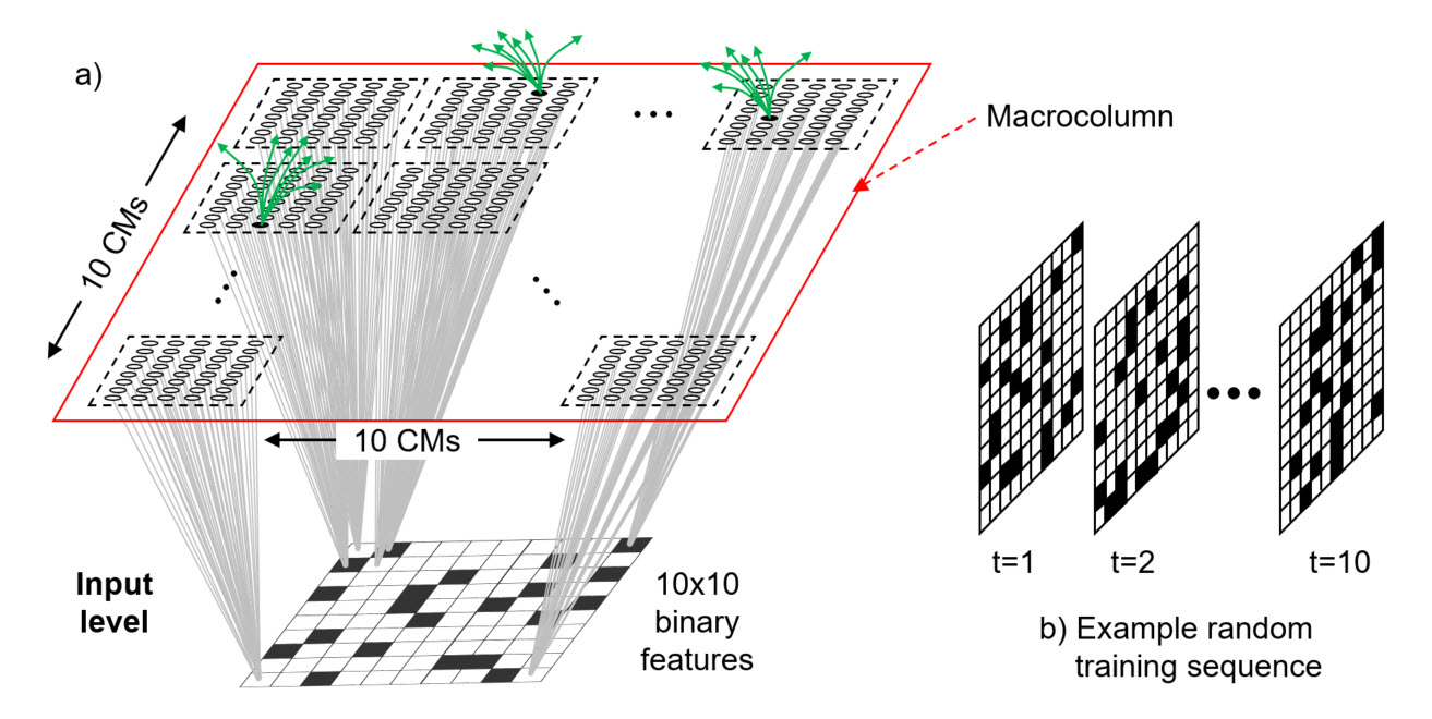
Figure 1: (a) The model has Q=100 WTA CMs, each with K=40 binary units. Horizantal weights suggested by green arrows. (b) Example of a training sequence used to test capacity. All sequences had 10 frames on which 20 binary features were randomly selected to be active. Thus the code that becomes active on each frame will consist of 20 winners, one in each of the 20 CMs whose corresponding input feature is active on that frame. All sequences are presented once.
A further point to be aware of here is that when we test for recall accuracy of the learned (stored) sequences, we actually prompt the model not with a sequence's first input pattern, but with the mac code that was assigned to that first input pattern during the learning trial. We then let the propagation of H signals from that first (T=1) code reactivate the next (T=2) code, and so on for the rest of the sequence. The accuracy measure reported is in terms of mac codes, not reinstated input codes. And, note that while we are assisting the model by telling it which unit to pick in each of the 20 active CMs on the first frame of each sequence, the accuracy measure does not include that first (T=1) code. After the first frame, all code activations depend only on the learned signals propagating via the H matrix.
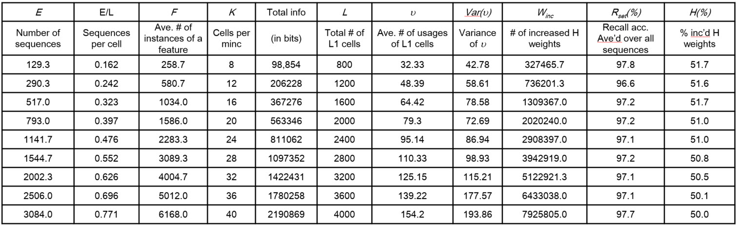
The Table and graphs below give the primary result which is that storage capacity (in terms of items, in this case, sequences):
- Increases superlinearly in the number of units (L), as shown in Table column "E" and chart a
- Increases linearly in the number of weights (chart b, which zooms in on the bottom two curves of chart a).
The table holds the data corresponding to the second lowest graph in chart a (labelled "UNC, STC=200", i.e., sequences were 10 frames long with 20 randomly chosen active features per frame; "UNC" means uncorrelated, which simply means that the active features were chosen uniformly at random on each frame). Each row represents the maximum number of such sequences storable while retaining average recall accuracy ≥ 97%, for a model of a given size. Model size, L and total number of weights (W, no column) systematically increases with row. Note: "L1" refers to input level, and "minc" ("minicolumn) is synonymous with "CM" (competitive module).
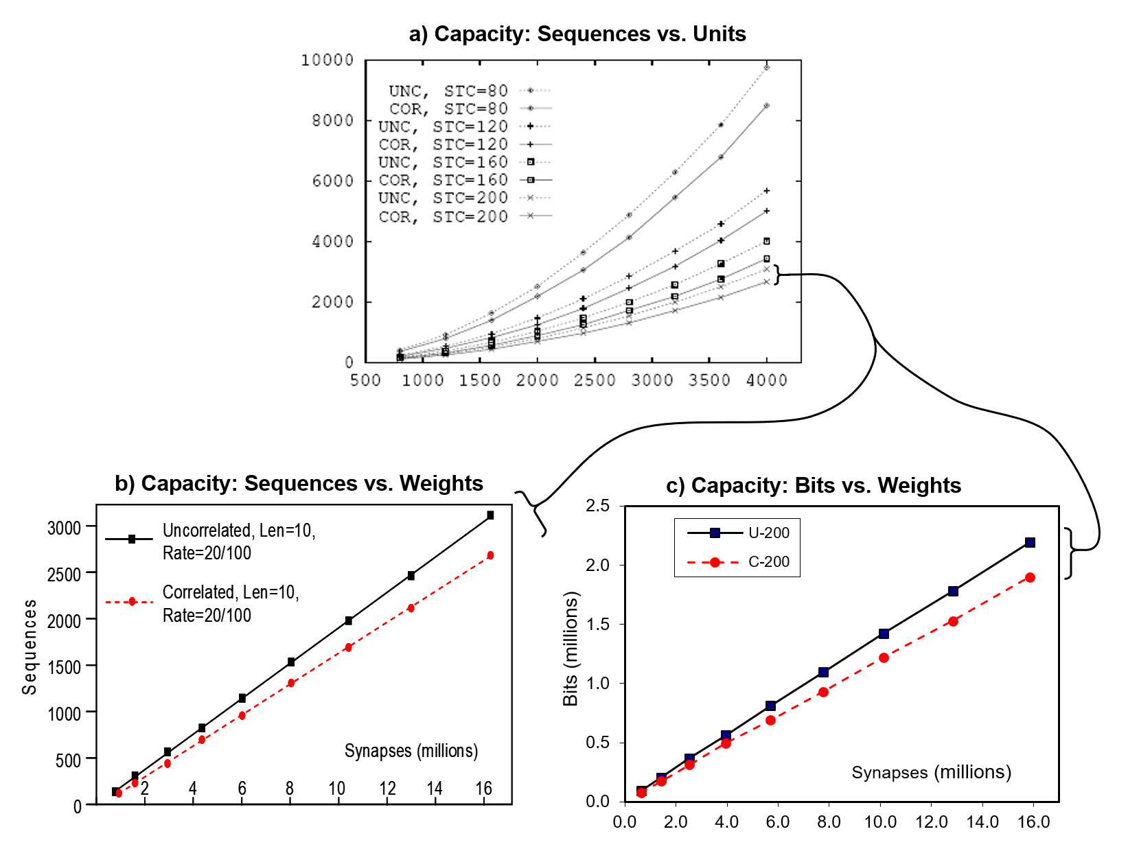
It is also very important that we also tested the case of complex sequences (here, called "correlated patterns", denoted "COR") corresponding to the dashed lines in charts (table not shown). For the correlated pattern experiments, we first generated a "lexicon" of 100 frames (each a random choice of 20 of 100 features). Then we generated the 10-frame training sequences by choosing randomly with replacement from the lexicon. Hence, each lexicon element occured approximately 1% of the time. This is important because the complex sequence case corresponds to natural lanquage lexicons. It is essential that any sequential/temporal memory be able to store massive numbers of sequences composed of frequently recurring items, as well as frequently ocurring sub-sequences of items. For the rightmost red dot in chart b above, about 2700 such complex squences were stored, each with 10 frames (total of 27,000 frames), meaning that in that case, the 100 lexicon items occurred an average of 270 times each.
In addition, chart c shows that capacity in bits increases superlinearly in the weights. The amount of information contained in each sequence (for the UNC case), was computed as shown below.
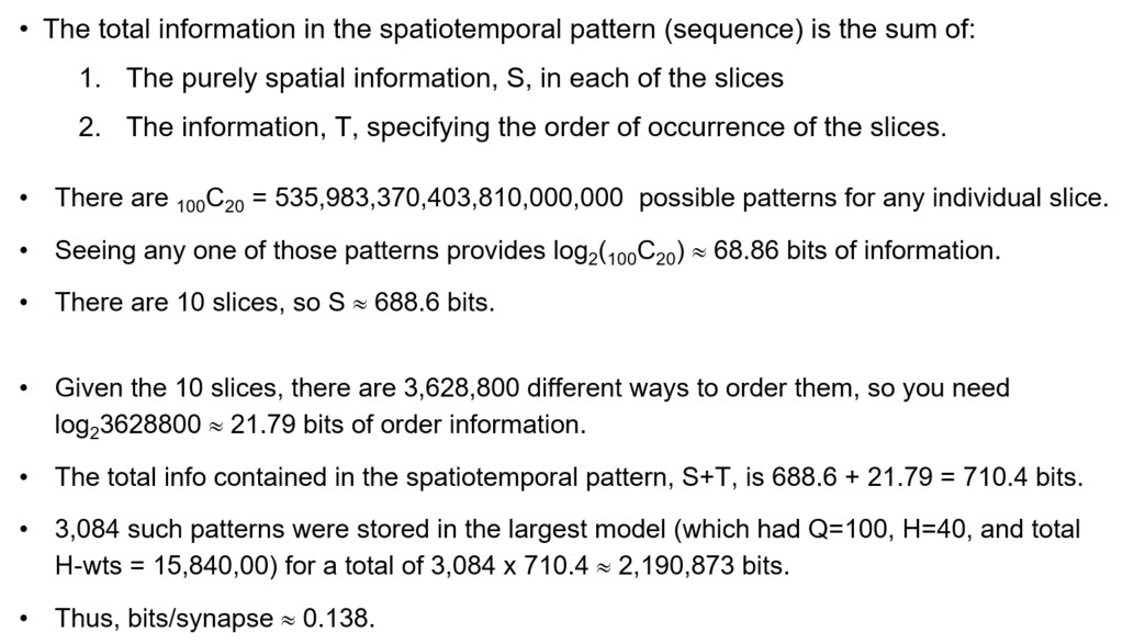
NOTE: This method overestimates the information contained in the whole set of sequences because it ignores the correlations (redundancies) amongst the set. We will attempt to find an approriate correction, but given that the sequences are completely random, we believe the overestimate may not be too severe. In any case, we believe that a bits/synapse value of this approximate value is quite tolerable for scaling to massive data sizes for at least two reasons: a) it comes in the context of a model with the more essential properties of being able to learn, with single trials, new sequences and retrieve the best-matching sequence in time that is fixed for the life of the model; and b) we expect the overall model bits/synapse value to increase significantly when hierarchy is leveraged. This latter point will be one of our research focuses going forward.