Sparsey Information Storage Capacity Study:
Study 2: Best-match Sequence Recognition
While Study 1 provides a baseline estimate of storage capacity, it does so in the context of exact-match retrieval. That is, we present exactly the same sequence on the test trial as on the training trial. In Study 2, we explore storage capacity in the context of best-match retrieval. We demonstrate best-match retrieval as follows. In each experimental run, we train the model on a set of random sequences. We then create a noisy version of each training sequence by randomly changing some fraction of the pixels in each of its frames. Figure 3 (middle) shows a typical training sequence. Figure 3 (top) shows the corresponding randomly produced noisy version of that sequence: one pixel was randomly changed in each frame, which actually yields two pixel-level differences between the original and the noisy frame. Each frame in the training set had between 9 and 12 active pixels, which yields noise levels from 2/9 = 22.2% to 2/12 = 16.7%. Figure 3 (bottom) shows a sequence produced from the middle one by randomly changing two pixels in each frame, which yields four pixel-level differences and thus noise levels, from 4/9 = 44.4% to 4/12 = 33.3%. In this study, we ran one series of experiments testing with the 1 pixel changed frames (columns 5-9 of Table 2) and one series testing with the 2 pixels changed frames (columns 10-14 of Table 2).
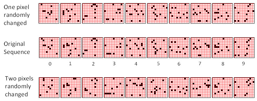
Figure 3: (Middle row) An example 10-frame training sequence used in Study 2. (Top row) A noisy version of the training sequence in which one pixel was randomly changed in each frame. The resulting frame has two pixel-level differences from the original. (Bottom Row) A noisy version of the training sequence in which two pixels were randomly changed in each frame.
Given the random method of creating individual frames of the training set and the high input dimension involved (144), if the fraction of changed pixels is small enough, e.g., < 10-20%, then the probability that a changed frame, x' will end up closer to (having higher intersection with) any other frame in the training set than to the frame, x, from which it was created, is extremely small. However, remember that Sparsey actually “sees” each input frame in the context of the sequence frames leading up to it, i.e., it computes the spatiotemporal similarity of particular moments in time (by virtue of its combining of U and H signals on each time step), not simply the spatial similarity between isolated snapshots. Thus, the relevant point is that the probability that a changed moment, e.g., [x',y',z'], with its exponentially higher dimensionality (1443), will end up closer to any other moment in the training set than to the moment, [x,y,z], from which it was created, is vanishingly small. (The notation [x,y,z], with z bolded, indicates the moment on which frame z is being presented as the third frame of a sequence after x and y have been presented as the first and second frames of the sequence.) This condition is required to validate the testing protocol/criterion described above, which compares the L1 code on each test frame to the L1 code on the corresponding training frame. Thus, if we can show that the model activates the exact same sequence of L1 codes in response to the noisy sequence, then we will have shown that the model is doing best-match retrieval.
Columns 5-9 of Table 2 show that the model is able to recognize a set of training sequences despite significant noise on every frame. As with Table 1, the absolute capacity increases with network size. For example, the network of Row 1 had 6,336 weights and showed good recognition of two 10-frame random sequences (containing 1,096 bits of information) despite 16.7%-22.2% noise on each frame, while the larger network of Row 4 had 39,168 weights and showed very good recognition for 10, similarly noisy, 10-frame sequences (5,563 bits of information), and so on. It is again the case that bits/synapse (B/S) seems to trend downward. However, as for Table 1, we believe this may be an artifact, and more importantly, even if there is some fundamental principle imposing a downward trend, it will ultimately prove slower than in these initial studies, and thus, the model will provide sufficiently high storage capacity to explain the apparent information capacity of biological brains and to provide an important technological building block for future computers. That is, what we are essentially testing in these studies are units that we postulate are analogous to cortical macrocolumns, of which human cortex contains on the order of two million. The capacities reported here, essentially for (very small instances of) a single macrocolumn must be seen in this light.
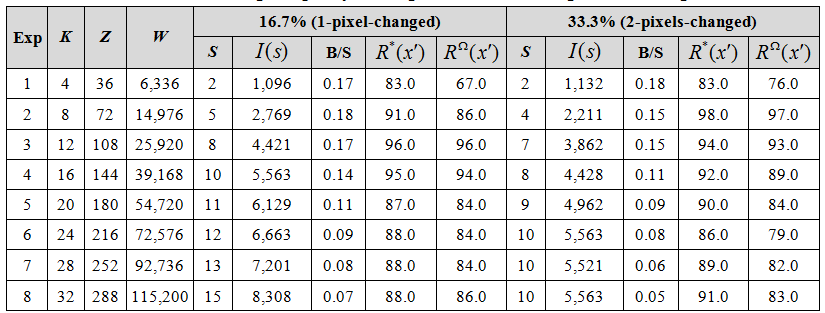
Key: As in Table 1, except that here we report only the total number of weights in the network, W. “B/S” is bits/synapse. S is the number of sequences in the training set. All sequences were 10 frames long. I(s) is the total information in the whole sequence set.
Columns 10-14 of Table 2 show that the model still performs well even for much larger per-frame noise levels. In these tests, which involved randomly changing two pixels on every frame, the frame-wise noise levels varied from 33.3% (on frames which had 12 active pixels) to 44.4% (on frames with 9 active pixels). A key point to note in Table 2 is that while the absolute capacities (and corresponding B/S values) are lower for the 2-pixel-changed series compared to the 1-pixel-chaged series, capacity still remains large. The primary reason for lower storage capacity in the 2-pixel-changed case is that because the test input frames are less similar to the training input frames (than in the 1-pixel-changed case), the r distributions from which winners in the CMs are chosen (Eqs. 7-8 of the CSA described in Tech Report 1) will be flatter, yielding more single-unit errors, thus reducing accuracy.
Table 3 gives the detailed (frame-by-frame) accuracies for all sequences for one run of Experiment 1 (top two rows) and one run of Experiment 4 (bottom 10 rows). The small network of Experiment 1 could store only two sequences while maintaining reasonably high recognition accuracy. The larger network of Experiment 4 (Z=144 L1 units and 39,168 weights) could store 10 sequences while maintaining very high accuracy. The rightmost column,![]() , is the average over all 10 frames of a given sequence presentation. It is important to note how the model fails as it is stressed by having to store additional sequences. Specifically, even as accuracy averaged over all sequences falls, a subset of the stored sequences is still recognized perfectly. This can be seen even in the small network example: Seq. 1 is retrieved virtually perfectly. Only a single unit-level error is made on frame 6. Seq. 2 starts out being recalled perfectly for the first few frames but then begins picking up errors in frame 4 and hobbles along for the rest of the sequence. Nevertheless, note that even on the last frame of Seq. 2, the L1 code is still correct in 5 of the 9 CMs. In Experiment 4, we see that 9 of the 10 sequences are recalled virtually perfectly, while one (Seq. 9) begins perfectly but then picks up some errors on frame 5 and then degrades to 0% accuracy by the last frame. It is also important to realize that while the model occasionally makes mistakes, it generally recovers by the next frame. In other examples (not shown here), the model can often recover from more significant errors. This topic will be discussed in Tech. Report 3.
, is the average over all 10 frames of a given sequence presentation. It is important to note how the model fails as it is stressed by having to store additional sequences. Specifically, even as accuracy averaged over all sequences falls, a subset of the stored sequences is still recognized perfectly. This can be seen even in the small network example: Seq. 1 is retrieved virtually perfectly. Only a single unit-level error is made on frame 6. Seq. 2 starts out being recalled perfectly for the first few frames but then begins picking up errors in frame 4 and hobbles along for the rest of the sequence. Nevertheless, note that even on the last frame of Seq. 2, the L1 code is still correct in 5 of the 9 CMs. In Experiment 4, we see that 9 of the 10 sequences are recalled virtually perfectly, while one (Seq. 9) begins perfectly but then picks up some errors on frame 5 and then degrades to 0% accuracy by the last frame. It is also important to realize that while the model occasionally makes mistakes, it generally recovers by the next frame. In other examples (not shown here), the model can often recover from more significant errors. This topic will be discussed in Tech. Report 3.
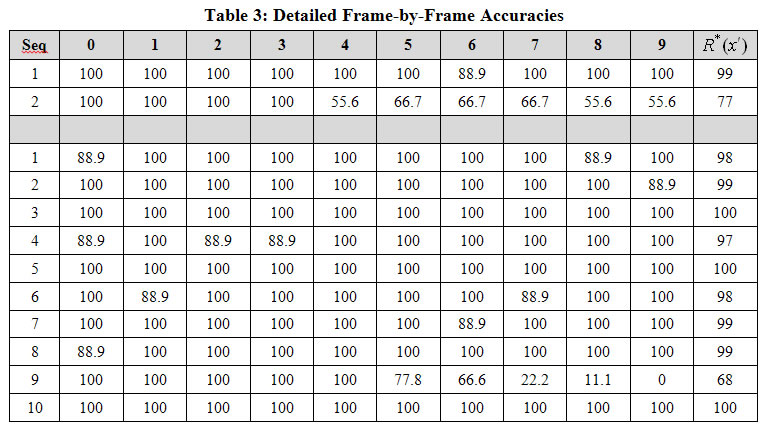
Key: All table cells give accuracies as percent. Last column is average of columns indexed 0-9.
Figure 4 shows the pair-wise L1 code intersections over the full set of frames (moments) experienced over all training and test episodes of the experimental run described in the top two lines of Table 3. Since there were two 10-frame sequences, this is a total of 40 frames (20 during learning and 20 during recognition). The upper yellow triangle shows the intersections between all codes assigned on the 10 frames of the training presentation of Seq. 1. Similarly for the other triangles down the main diagonal. The top value the green triangle (row 20, col. 0) shows that L1 code “20”, i.e., the code activated on the first frame of the test presentation of Seq.1' (which is the 1-pixel-changed version of Seq. 1) intersects completely (in all Q=9 CMs) with L1 code 0, i.e., the code activated on the first frame of the training presentation of Seq. 1. Similarly, for codes, 21 and 1, 22 and 2, etc. Reading down the minor diagonal (between the red lines) tells how well the model does: perfect recognition of all noisy frames of all sequences would yield “9”s all the way down.
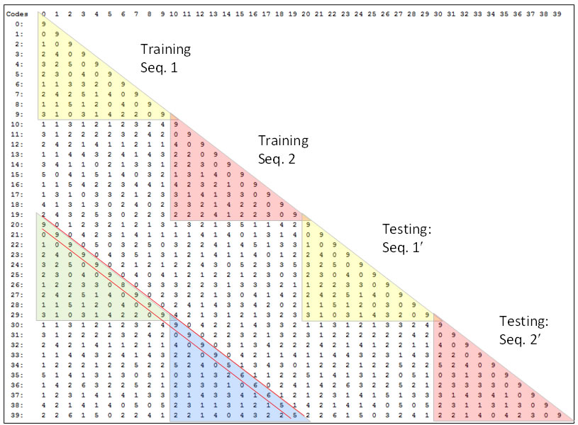
Figure 4: Pair-wise intersections of all L1 codes assigned in one run of the 1-pixel-changed testing condition for the smallest model tested, which had Q=9, K=4, and 6,336 weights.
When each frame is presented during a recognition test trial the likelihoods of all codes stored during the learning trial are formally evaluated. They are evaluated in parallel by the constant-time code selection algorithm (CSA). However, at no point does the model produce explicit representations of the likelihoods of the individual codes (hypotheses) stored. Such an explicit representation, e.g., a list, of likelihoods would constitute a localist representation of those likelihoods. What the model actually does is make Q draws, one in each CM. However, the net effect of making these Q draws (soft-max operations) is that a hard-max over all stored hypotheses is evaluated. This is true whether the model has stored a single 5-frame sequence, or a single 500-frame sequence, or 100 5-frame sequences. And crucially, because the numbers of CMs, and thus units, and weights, are fixed, the time it takes to make those Q draws remains constant as additional codes (hypotheses) are stored.
What the results in this report say is that that hard-max, i.e., the max-likelihood hypothesis, is returned with probability that can be very close to 1 if the amount of information (i.e., number of hypotheses) stored remains below a soft threshold, and which decreases as we move beyond that threshold. For example, looking at Table 3, we see that for the Experiment 4 (bottom 10 rows), the model chooses the correct, i.e., maximum likelihood, hypothesis on almost all of the 100 frames (moments) of the test phase. These are 100 independent decisions, in each of which, all 100 stored hypotheses had some non-zero possibility of being activated. Yet, almost all 100 whole-code-level decisions were correct. And, at the finer scale of the individual CMs, where the actual decision process, albeit a soft decision process, takes place, almost all (861) of the 900 decisions were correct.
Table 4 shows what happens when we move past or perhaps through, the aforementioned soft threshold. In these two experiments, we again used the network with 39,198 weights and the 1-pixel-changed test, but the training/test sets contained 11 sequences (for the experiment reported in the upper 11 rows) and 12 sequences (for the experiment reported in the lower 12 rows), compared to only 10 in Experiment 4 reported in Table 3. For the 11-sequence case, the model still performs very well on six of the sequences, but adding another sequence degrades performance substantially more.
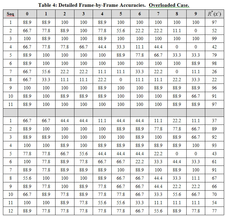
Key: All table cells give accuracies as percent. Last column is average of columns indexed 0-9.