Sparsey Information storage capacity study:
Study 1: exact-match sequence recognition
The goal of this study was to generate a preliminary quantitative analysis of the model’s storage capacity. To do this, we focused on a small model instance with one internal level and a 12x12 binary pixel input surface. To quantify capacity, we created random sequences of 12x12 frames. The first 30 frames of one such sequence, S1, are shown at the top of Figure 1. Each frame was produced by randomly choosing between 9 and 12 of the 144 pixels to be 1 and the rest 0. Thus, S1 is essentially a sequence of white noise frames. We chose to test capacity with random sequences because they have the minimum expected correlation over any single sequence and over any set of such sequences. This facilitates quantifying the amount of information (in bits) contained in each sequence and in each set of sequences. The information calculation method is given shortly.
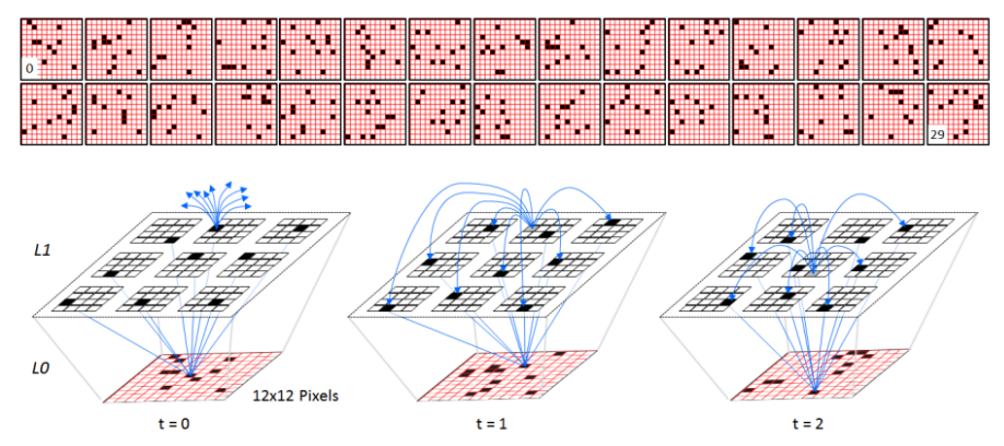
Figure 1: (Top) The first 30 frames of a randomly generated sequence, S1, used to test the model’s storage capacity. (Bottom) One of the 2-level model instances used in Study 1, shown on the first three frames of S1. The internal level, L1, consists of Q=9 WTA competitive modules (CMs), each consisting of K=16 binary units (neurons). The U and H weight matrices are complete, yielding a total of 39,168 weights (connections): blue lines show a tiny sample of the weights.
Figure 1 (bottom) depicts a 2-level model instance used in this study at successive moments in time, specifically while processing the first three frames of S1. The internal level, L1, consists of Q=9 winner-take-all (WTA) competitive modules (CMs), each consisting of K=16 binary units (neurons). The spray of blue arrows at t=0 indicates the initiation of horizontal (H) signals from an L1 unit activated at t=0, which arrive (recur) back to L1 at t=1. That unit is shown in gray at t=1 (indicating it has turned off) and the set of H weights that are increased from that unit onto the units active at t=1 are shown as completed blue arrows. The other 8 L1 units active at t=0 will also increase their weights onto the L1 units active at t=1. Thus a total of 9x8=72 H weights are increased at t=1 (units do not have H weights onto the other units in their own CMs). This form of temporal chaining occurs from each code onto the successor code throughout the duration of the sequence, e.g., we show more H learning at t=2, from the winner in the central CM at t=1 onto the winners at t=2. Also note that in general, L1 units simultaneously receive U inputs from the currently active input and H inputs from the previously active L1 code, thus simultaneously updating subsets of their afferent U and H weights, and thus acquire spatiotemporal receptive fields (RFs).
Each individual experiment of this study consists of a single unsupervised training presentation of a sequence during which a spatiotemporal memory trace—i.e., a chain of SDR codes in the internal level—is formed, and one recognition test presentation. Recognition accuracy is computed by comparing the similarity of the SDR code active on each frame t of the recognition presentation to the code that was active on frame t of the training presentation. Eq. 1 defines the similarity, ![]() , of code
, of code ![]() active on frame t of sequence x to code
active on frame t of sequence x to code ![]() active on frame t of sequence x' as the size of the intersection of the two codes divided by code size, which, because all codes consist of one winner per CM, is fixed at Q. Here,x and x' refer to training and test presentations, respectively, of a given sequence.
active on frame t of sequence x' as the size of the intersection of the two codes divided by code size, which, because all codes consist of one winner per CM, is fixed at Q. Here,x and x' refer to training and test presentations, respectively, of a given sequence.
| (Eq. 1) |
We compute the recognition accuracy of a whole sequence in two ways. The first,![]() , is just the average of
, is just the average of ![]() over all T frames of a sequence x', as in Eq. 2. The second,
over all T frames of a sequence x', as in Eq. 2. The second,![]() , is just the accuracy on the final frame of sequence x', as in Eq. 3, where T-1 is the index of the last frame. Note that “x” is omitted from the notations for these and subsequent accuracy measures since it is specifically the test sequence, x', whose accuracy is measured (though it is implicitly with respect to the corresponding training presentation). The first, more stringent, measure is more relevant in applications where it is important for the model to maintain the correct hypothesis as to the identity/category of an input sequence throughout its duration. The second measure is more relevant in applications where all that matters is that the model comes up with the right answer by the time an input sequence completes.
, is just the accuracy on the final frame of sequence x', as in Eq. 3, where T-1 is the index of the last frame. Note that “x” is omitted from the notations for these and subsequent accuracy measures since it is specifically the test sequence, x', whose accuracy is measured (though it is implicitly with respect to the corresponding training presentation). The first, more stringent, measure is more relevant in applications where it is important for the model to maintain the correct hypothesis as to the identity/category of an input sequence throughout its duration. The second measure is more relevant in applications where all that matters is that the model comes up with the right answer by the time an input sequence completes.
 |
(Eq. 2) |
| (Eq. 3) |
Table 1 shows how the model’s information storage capacity in bits increases with model size. The major determinant of model size is the number of weights (synapses), so we report storage capacity in bits per synapse. In this series of experiments, we varied model size specifically by increasing K, while holding Q=9 constant. Of course, as K increases, the numbers of U and H weights increases (H increases quadratically). Each row reports the data for one experimental configuration, i.e., model size, but averaged over 10 runs of that experiment. As model size grows, the length of the sequence used to test it increases. The sequence used in Exp. 1 consisted of the first 20 frames shown in Figure 1 (top). Actually, a master sequence of 250 frames, with between 9 and 12 active pixels per frame was generated at the outset. For progressively larger model sizes, we used progressively longer prefixes of that master sequence. Thus, Exp. 2 used the first 60 frames of the master sequence, Exp. 3, the first 100, etc.
It is important to realize that the model is learning these long sequences, up to 210 frames long in Exp. 8, with single trials. Also, the results in Table 1 are averages over 10 runs of any given experiment; the model achieved perfect 100% recognition accuracy on many individual runs across all experiments. For example, the first 5 L1 codes (and corresponding inputs) of a 120-code-long memory trace learned perfectly on one run of Exp. 4 are shown in Figure 2. That is, on each of the 120 frames of the recognition presentation, the same 9 winners were chosen as on the corresponding frame of the learning presentation. Figure 2 also shows a small sample of some of the U and H connections increased on each frame. On each recognition frame, it is the multiplicatively combined U and H inputs to L1 (Step 2.5 of the generalized CSA in Tech. Report 1) that determines the winning code.
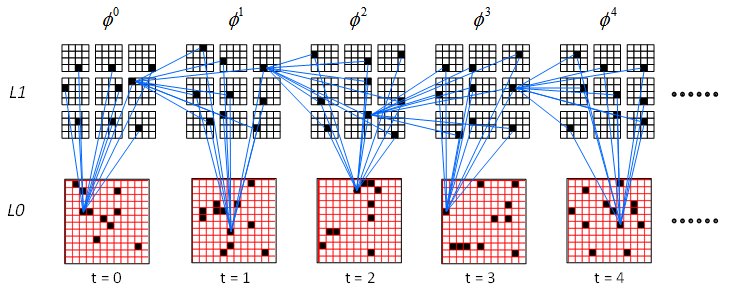
Figure 2: The first 5 L1 codes (and corresponding inputs) of a 120-code-long memory trace learned perfectly on one run of Exp 4.
Table 1: Storage Capacity Scaling: Exact-Match Recognition Testing
| Exp. | T | I(s) | K | Z | U | H | U+ | H+ | Bits / Synapse | ||
|---|---|---|---|---|---|---|---|---|---|---|---|
| 1 | 20 | 1,114 | 4 | 36 | 5,184 | 1,152 | 1,427 | 666 | 0.176 | 85.0 | 62.3 |
| 2 | 60 | 3,459 | 8 | 72 | 10,368 | 4,608 | 3,834 | 2,287 | 0.23 | 86.2 | 54.4 |
| 3 | 100 | 5,828 | 12 | 108 | 15,552 | 10,368 | 6,244 | 4,473 | 0.22 | 87.8 | 44.3 |
| 4 | 120 | 7,062 | 16 | 144 | 20,736 | 18,432 | 7,969 | 6,065 | 0.18 | 86.2 | 35.6 |
| 5 | 140 | 8,245 | 20 | 180 | 25,920 | 28,800 | 9,710 | 7,627 | 0.15 | 84.0 | 72.3 |
| 6 | 160 | 9,449 | 24 | 216 | 31,104 | 41,472 | 11,008 | 8,804 | 0.13 | 85.2 | 48.9 |
| 7 | 180 | 10,629 | 28 | 252 | 36,288 | 56,488 | 13,291 | 1,118 | 0.12 | 97.5 | 92.2 |
| 8 | 210 | 12,440 | 32 | 288 | 41,472 | 73,728 | 14,355 | 11,209 | 0.11 | 76.5 | 67.8 |
Key: The R measures (defined in the text) are in %. T is sequence length in frames. The I(s) calculation (in bits) is defined in Eqs. 4-6. Z= Q x K is the total number of L1 units. U is the number of bottom-up (U) weights from L0 to L1. H is the number of horizontal (H) weights in L1. U+ and H+ are the numbers of U and H weights increased on the training presentation. U+, H+, Bits/Synapse,![]() , and
, and![]() , are averages over the 10 runs of an experiment.
, are averages over the 10 runs of an experiment.
We compute the total bits in a sequence as follows. As noted above, each sequence frame was produced by randomly selecting B (9 <= B <= 12) of the 144 pixels to be 1. The amount of spatial information![]() in frame t is therefore just the base 2 log of the number of ways of choosing B(t) units from 144 units. Because the frames are chosen independently of each other, we ignore as negligible the chance-level pixel-wise correlation across frames that will accrue with longer sequences. Thus, the spatial information contained in a whole sequence s is just the sum of
in frame t is therefore just the base 2 log of the number of ways of choosing B(t) units from 144 units. Because the frames are chosen independently of each other, we ignore as negligible the chance-level pixel-wise correlation across frames that will accrue with longer sequences. Thus, the spatial information contained in a whole sequence s is just the sum of ![]() over all t, as in Eq. 4. We can then separately calculate the amount of temporal order information
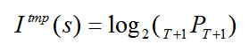
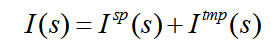
over all t, as in Eq. 4. We can then separately calculate the amount of temporal order information![]() in s as the base 2 log of the number of permutations of the T frames of s, as in Eq. 5. The total bits of information, I(s), is the sum of the spatial and temporal information components (Eq. 6).
in s as the base 2 log of the number of permutations of the T frames of s, as in Eq. 5. The total bits of information, I(s), is the sum of the spatial and temporal information components (Eq. 6).
 |
(Eq. 4) |
 |
(Eq. 5) |
 |
(Eq. 6) |
The increasing total bits stored [I(s)] with size (Total wts, which is the sum of columns, “U” and “H”) can clearly be seen. However, these data must still be considered rough estimates for several reasons including the following.
- In moving from one model size to the next larger, we increased sequence length, T, typically by 20 and began doing test runs to verify that the more stringent capacity measure,
 , was in the ballpark of 85-90%. If it was, then we would perform 10 runs with that sequence and report the average in Table 1. Otherwise, we would chop 10 frames off the sequence and test again. Ideally, we should search more finely over sequence length.
 - Given the probabilistic way in which winners, and thus whole SDR codes, are chosen during recognition, we should probably be averaging over at least 100 runs, not 10.
- We did not perform any systematic search through parameter space in each experiment. Rather, the same parameters, except for K, are used in each experiment. While there are theoretical reasons for believing that the parameters used should yield large capacity across very wide ranges of other model parameters, in particular, K, a systematic search should be performed. The simulation’s automatic testing functionality is currently being upgraded to address these issues.
- The fraction of weights increased trends downward from 30-40% in Exps. 1-5 to 25-30% in Exps. 6-8. We are not sure why this is happening yet, but from basic information principles, we should expect the maximal amount of information storable in a network of binary weights to correspond to condition in which about 50% of the weights have been increased. This suggests that the estimates of I(s) and of bits per synapse in Table 1 may be low. We will investigate this issue, going forward.
- The capacities reported in the table are somewhat inflated because they do not factor in the recognition accuracies. The same algorithm, the CSA (see Tech Report 1), is used on both learning and recognition. During recognition, on each frame, in each L1 competitive module (CM), the CSA chooses a winner from a distribution over that CM’s units. Even if the distribution is very peaked over the correct unit, there will still be a chance of error since, particularly since recognition is being tested after a lot of frames have been stored, all of the other units in the CM will generally also have non-zero probability of being chosen. That is, as emphasized in Tech Report 1, the CSA does not simply pick the hard max from the distribution, but rather the softmax. Once the learning has been done, choosing winners by softmax must be less optimal (i.e., it can only entail more errors) than choosing by hard max. This suggests that the capacity estimates of Table 1 might be considerably lower than could be achieved if the hard-max method was used during recognition. We will implement the hard-max method and report those results in a subsequent report.
- Bits per synapse seems to trend downward with larger networks. We do not have an immediate explanation for this apparent trend. In fact, we suspect it is an artifact due to the interactions of the important effects/principles described in the other items of this list, amongst others. In light of those effects, a statistically more robust battery of experimentation is clearly needed to really see how these numbers trend. In any case, the theoretical maximum number of bits storable per binary synapse is approximately ln(2)≈0.693. The capacities in Table 1 are within an order of magnitude of the theoretical maximum and further, possibly substantial, improvements are still likely, e.g., choosing by hard-max during recognition, etc.
Despite these imperfections, we believe that the results in Table 1 demonstrate sufficiently high storage capacity in the context of exact-match retrieval to warrant shifting focus to the next issue, which is demonstrating such high capacity in the context of best-match retrieval (which is the focus Study 2).
Beyond the points made in the list above, there are at least two more important principles that will be at play in a more comprehensive storage capacity analysis.
- Natural input domains have a great deal more correlation (redundancy), and thus a lot less information, than the random sequences used in this study. Given a sequence length, T, and an average coding rate (fraction of active pixels per frame), C, a sequence derived from a natural input domain should contain much less information than a random sequence of the type used in Study 1. This is why a relatively small overcomplete basis can generally do a very good job of representing, to close approximation, any future input from the domain. With this in mind, testing with random sequences should be viewed as a “stress test” of storage capacity and we should expect the capacities reported, e.g., in Table 1, to be lower bounds on the capacities that would be realized for real domains. In fact, we are not seeing this yet in our data, e.g., in comparing Study 1 (Table 1) to Study 3 (Table 5). However, we believe this is due to the reasons given in the prior list and to the fact that the studies in this report do not involve multi-level models and so cannot leverage the compression possible with an explicit (structural) hierarchy, as mentioned in point 2 below.
- The effect of hierarchy, and more specifically, of explicitly representing an input domain at multiple spatial and temporal scales (i.e., levels) where the representations at adjacent scales are linked and act in coordination should allow a given set of inputs, in particular, naturalistic inputs, to be represented with fewer total connections than a non-hierarchical (1-level, flat) representation.