Preliminary MNIST Results
This page describes performance of a 2-level (non-hierarchical) version of Sparsey on MNIST. The first series of experiments involved a subset containing 9,000 MNIST samples (900 per class). The net was trained on 200 samples per class and the test set varied from 100 to 700 examples of each class. The original 28x28 gray-level images were scaled to 16x24, binarized, and skeletonized, using ImageJ, resulting in images such as in Figure 1. The model used is shown in Figures 2 and 3 and the results are reported in Table 1. Larger studies training on 800 samples per class and testing on up to 50,000 samples (5,000 per class) are described in Table 2.
The main result of the first series is that the 2-level Sparsey (one internal level) is able to achieve 91% recognition accuracy on MNIST test samples after doing extremely fast single-trial learning (220 secs. on a single thread) on a small subset of the MNIST data, i.e., only 200 instances per class. As Table 1 shows, recognition accuracy drops slowly as we increased the test set from 100 samples per class to 700 samples per class. In fact, in the larger tests of Table 2, class accuracy remains constant for all test set sizes. We emphasize that most other MNIST solutions reported in the literature required training on most of the samples (~60,000) and testing on a much smaller subset (~10,000). However, the ML community increasingly acknowledges that human learning generally relies on far fewer training samples and far fewer trials than have typically been used. In any case, the class accuracy numbers reported in Table 2 are for much larger test sets than are generally reported for MNIST.
While this main result, 91% accuracy, is less than state-of-art (>99%), it must be considered in light of several other crucial points.
- Sparsey uses only unsupervised Hebbian learning (It also has passive decay but that has little effect in these particular studies). No computation of gradients or generation of samples as in MCMC is needed.
- The units (neurons) are binary and the weights are effectively binary.
- The learning is single-trial (one shot).
- Learning is "fixed-time", i.e., the time it takes to learn each new sample remains constant over the life of the system.
- The learning in this example took 220 sec. on a single CPU (Xeon 3.2 ghz)...with NO MACHINE PARALLELISM !
- Testing is also "fixed-time" and took 90 sec. for the 1000 test samples.
- The Java software used here includes extra housekeeping and stat-gathering processing and could likely be made faster by at least 1-2 orders of magnitude even without resorting to any sort of machine parallelism. However, we emphasize that Sparsey's computations are spatially and temporally local and could realize much greater additional speedup from machine parallelism, e.g., memristor.
- As Figure 1 shows, only simple binary pixels are used as input; no higher-order features of any kind are used to make the recognition task easier.
- Many avenues are available for improving these results. Most notably, we still have huge regions of the model's full parameter space to explore. Second, this model was non-hierarchical. We are currently exploring models with more levels as well, but due to the complex interactions of the numerous parameters, the multi-level models' performance is still lower than the 2-level model. Nevertheless, we are confident that the recursive, parts-based decomposition of the space will yield the highest possible accuracy. In addition, we expect that using other sorts of more informative features will also yield higher accuracy. Our primary goal has always been to understand how actual biological intelligence works. Since biological brains ultimately have only the raw pixels as inputs, we have spent almost no time exploring any more infomative features to aid recognition.
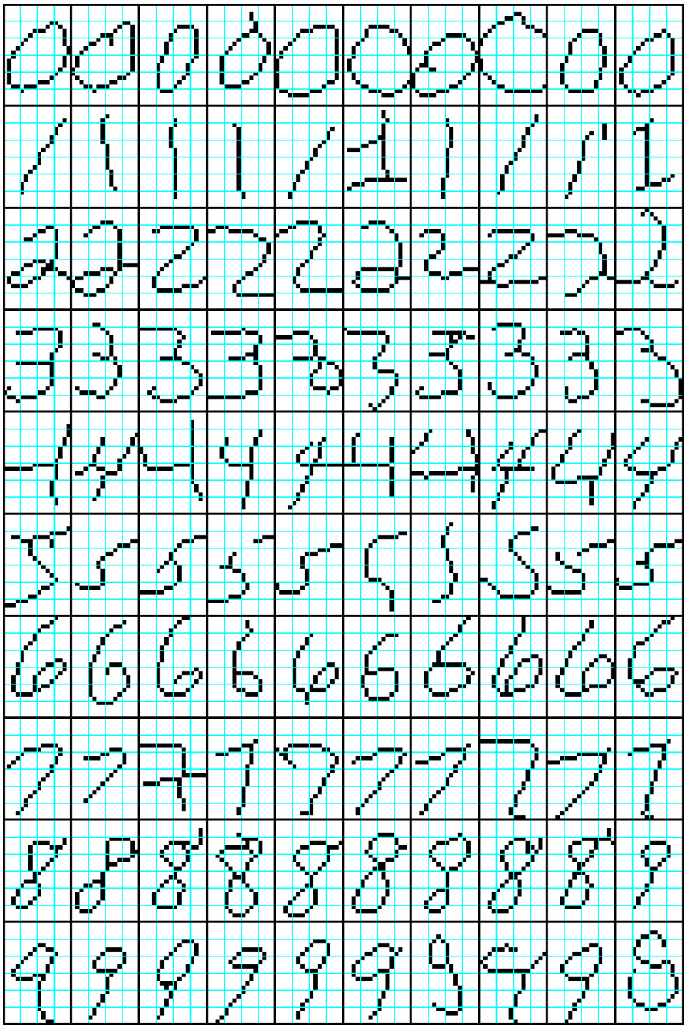
Figure 1: 10 samples from each of the 10 MNIST classes after preprocessing. Original MNIST images were changed to 16x24 pixels, binarized, and skeletonized. The blue squares are 4x4 pixels.
The Sparsey model instance used for the studies in Table 1 consisted of one internal level consisting of 21 x 32 = 672 macs as shown in Figure 2. Every mac had Q=11 WTA competitive modules (CMs), each with K=9 binary cells. There were a total of 1.54 million wts, all of which were from the pixels comprising the input level (L0) to L1. In this particular case, an example of digit "5" is being presented and 77 of the 672 macs are activating in response (rose shaded) because the numbers of active pixels in their respective RFs meets their parametrically determined constraints. Figure 3 shows the RFs for several of the active macs. For example, the rightmost mac for which the RF is shown activates if exactly 3 out of the 14 pixels comprising its RF are active, whereas the mac at right center activates if exactly 6 out of the 51 pixels comprising its RF are active. The blue lines show a subset of the U wts connecting pixels in the RF to one of the cells (not visible) in the mac.
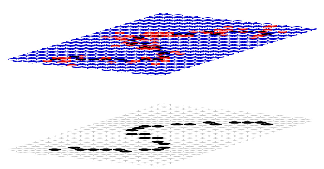
Figure 2: The Sparsey model that was used in these Studies. It had one internal level consisting of 21 x 32 = 672 macs. Every mac had Q=11 WTA competitive modules (CMs), each with K=9 binary cells. There were a total of 1.54 million wts, all of which were from the pixels comprising the input level (L0) to L1.
Figure 3 repeats Figure 2 but highlights the RFs of several of the active L1 macs. In this particular model, the RFs are highly overlapped: neighboring macs may have over 90% of their pixels in common. But the sizes of the RFs and the numbers of pixels required to activate the macs differ from one mac to the next. The effect of these variations is that every active pixel generally participates in activating several of the overlying macs and is thus represented multiple times and in multiple contexts at the internal level. This is a kind of inter-mac overcompleteness which is in addition to the intra-mac overcompleteness.
Although it cannot be seen in thise figures, the activation of each active mac takes the form of a sparse set of Q=11 coactive cells (one winner in each of the Q=11 CMs). Thus, there are actually 77 x 11 = 847 active cells in L1. Although also not shown here, all of the 672 x 11 x 9 = 66,528 cells comprising L1 are connected to a set of 10 class label cells. These weights are increased during learning and during recognition, the label cell with the maximum summation is the winner.
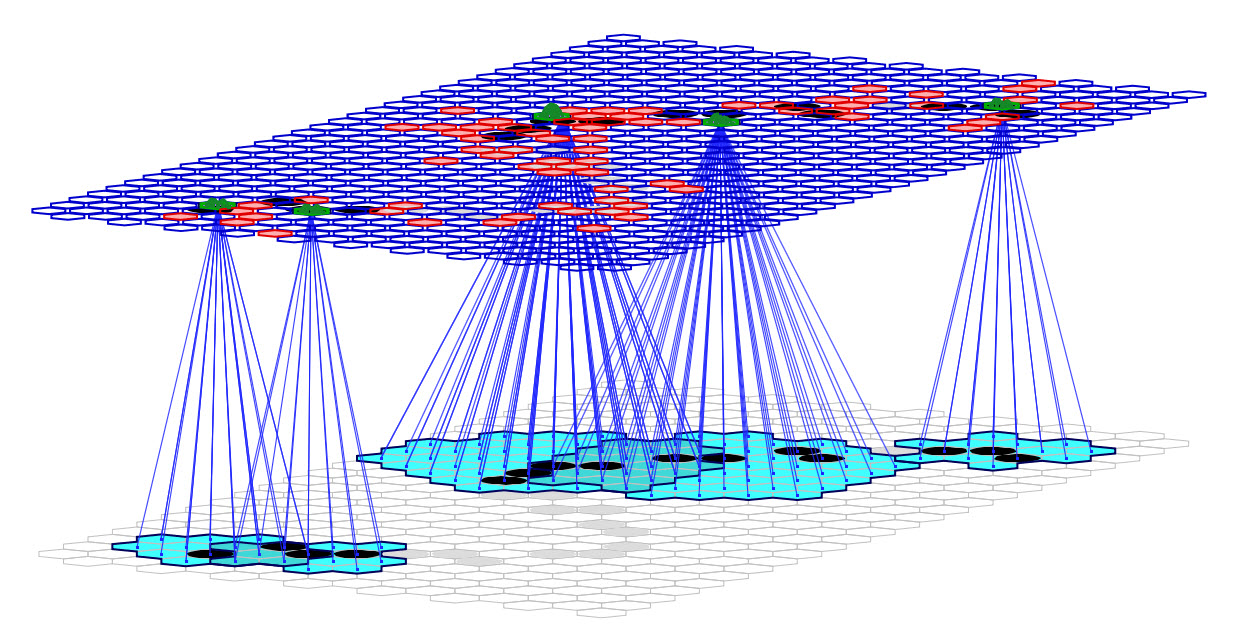
Figure 3: The Sparsey model that was used in these Studies with the RFs of several macs highlighted.
Table 1: MNIST Recognition Accuracy
| Exp. | Train Samples / Class | Test Samples / Class | Acc. (%) |
|---|---|---|---|
| 1 | 200 | 100 | 91 |
| 2 | 200 | 200 | 89 |
| 3 | 200 | 400 | 88 |
| 4 | 200 | 700 | 87 |
Table 1 shows the results of four experiments involving progressively larger test sets. The model was trained once and the four tests were run using that same model. Two key parameters for this model were: a) the distribution of values determining how many active cells are needed to activate a mac (the π parameter) from which draws were made during model construction; and b) the distribution of values determining the radii of (and thus, the numbers of pixels comprising) the RFs from which draws were made. These were [0.115, 0.120, 0.130, 0.160] and [3.8, 4.0, 4.2, 4.4, 4.6], respectively. The latter distribution led to average RF size of 31.4 pixels. In conjunction with the π parameters, these ensured that all active input pixels, i.e., input features, of all train and test images participated in causing at least one mac to activate. Thus, all information present in the input had an influence on the classification behavior. In addition, the average number of macs active across all training samples was 80 and the average number of unique codes stored in each mac was 232: in other words, the average basis size was 232. Finally, a maximum of 33% of a mac's afferent wts (from L0), the saturation threshold, were allowed to be set high.
Table 2: MNIST Recognition Accuracy
| Exp. | Train Samples / Class | Test Samples / Class | Acc. (%) |
|---|---|---|---|
| 1 | 800 | 500 | 89 |
| 2 | 800 | 1000 | 89 |
| 3 | 800 | 2000 | 88 |
| 4 | 800 | 3000 | 89 |
| 5 | 800 | 5000 | 89 |
Table 2 shows results involving much larger test sets, indeed testing on up to 50,000 of the 70,000 MNIST samples. The same model, trained on only 800 samples per class, was used in all experiments. The π and RF radii parameters were [0.115, 0.120, 0.130, 0.160] and [2.2, 3.1, 4.1, 3.1, 4.1], respectively. The latter distribution results in smaller average RF size than for the model in Table 1. However, for this model, Q=16 and K=11, resulting in a total of ~3.7 million weights. Here, the saturation threshold was 18%. Training on 8000 samples takes 25 minutes (on a single CPU thread), though again, we expect at least 1-2 orders of magnitude speed-up should be possible via software optimizations. Moreover, we expect that significantly smaller models (fewer macs, smaller Q and K) could reach the same classification performance and this will be a subject of continued parameter search.
The main point about Table 2 is that classification accuracy remains constant as we scale the test set from 5,000 samples (500 per class) to 50,000 (5,000 per class).
We emphasize that the we are still far from having a complete understanding of the optimal values of the model's numerous parameters, including the dimensions of the L1 array of macs, the RF sizes, the π distributions, Q, K, and many others.