Overview of Sparsey® Model
Note: the most comprehensive description of Sparsey is in the Frontiers in Neuroscience article, Sparsey: Event recognition via deep hierarchical sparse distributed codes. This page highlights some of its main architectural and processing properties.
In general, a Sparsey model instance is a multi-level hierarchical (or heterarchical) network comprised of numerous macs whose comprising units (neurons) communicate with each other via bottom-up (U), horizontal (H), and top-down (D) synaptic matrices. Figure 1 shows a tiny 4-level instance with only 21 macs. We emphasize that very few other neural models explicitly enforce structural/functional organization at the mesoscale, discussed here.
A Sparsey mac consists of Q winner-take-all (WTA) competitive modules (CMs), each consisting of K binary units. When a mac becomes active, one unit in each CM is activated (how unit is selected, i.e., the code selection algorithm (CSA), is described in Rinkus 2010 and 2014) and at right. The set of Q winners is a sparse distributed representation (SDR), a.k.a., sparse distributed code (SDC). It also qualifies as a cell assembly. We often refer to them as mac codes. Q and K can vary by level and from one mac to another within a level.
In research thus far, we have used the simplification that all units in a mac have the same exact receptive field (RF). This applies to U-inputs and D-inputs (Figure 1) and H-inputs (Figure 2). Figure 1 shows the full U (blue) and D (magenta) afferent matrices leading to the active code (black cells) in one particular L1 mac: every cell has exactly the same U and D RF. Figure 2 shows a fraction (for clarity) of the afferent H wts (green) to the active code: every cell receives input from every cell in each of its six neighboring macs and every cell in its own mac except from those in its own CM (cyan indicates the source H field of macs; purple indicates a mac that is both in the source field and active). Thus, when in learning mode, when a mac code activates and the afferent weights leading to the mac's units are increased, that code becomes the representation (code) of the total input present in the mac's total RF.
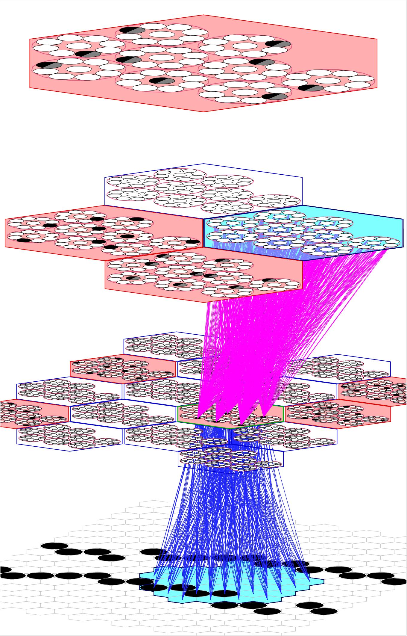
Figure 1: A small Sparsey instance with three internal levels and 21 macs. The afferent U (blue) and D (magenta) wts leading to the active (black) cells in one L1 mac are shown, indicating that all cells in a CM have exactly the same U and D receptive fields (RFs).
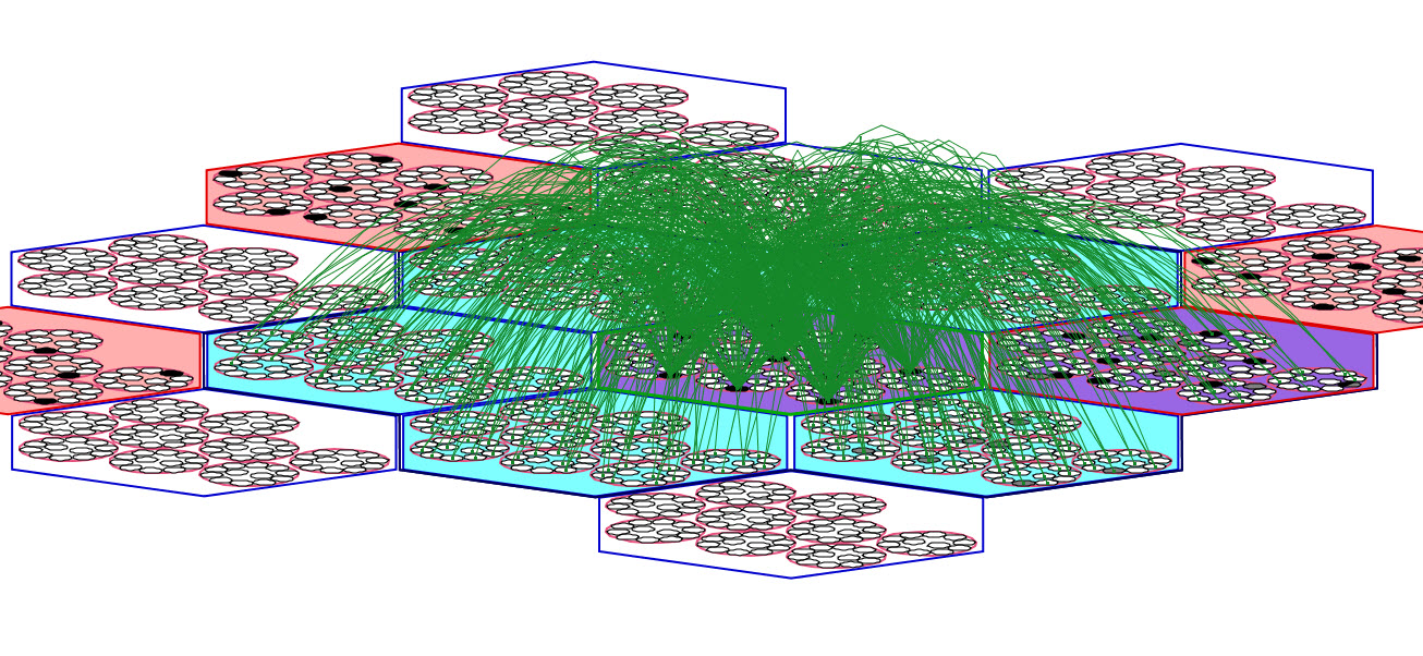
Figure 2: Zoom-in of same L1 mac showing that every cell has the same H RF as well. Only a fraction of the H wts (green) are shown.
The learning, i.e., the association of the input pattern to the code, is made with full strength with a single-trial. A weight's strength decays back towards zero over time. If another pre-post coincidence occurs within a time window, the weight is increased to the max again and another property, its permanence, is increased, which decreases its decay rate. Thus, Sparsey's learning law is purely local (in space and time): essentially, Hebbian-type learning with decay.
Since the H and D weights provide recurrent pathways and are defined to deliver signals from the previously active codes in their source (pre-synaptic) fields, a mac's input is generally spatiotemporal. We refer to such inputs as "moments", as in particular moments in time.
Figure 3 illustrates the core Sparsey circuit [i.e., the circuitry that implements the "Code Selection Algorithm" (CSA)] in a minimal instance model with two internal levels with one mac at each level. Each mac has Q=4 CMs, each with K=3 neurons. The afferent U (gray), H (green, only a small representative sample shown), and D (magenta) matrices are shown for the L1 mac (yellow).
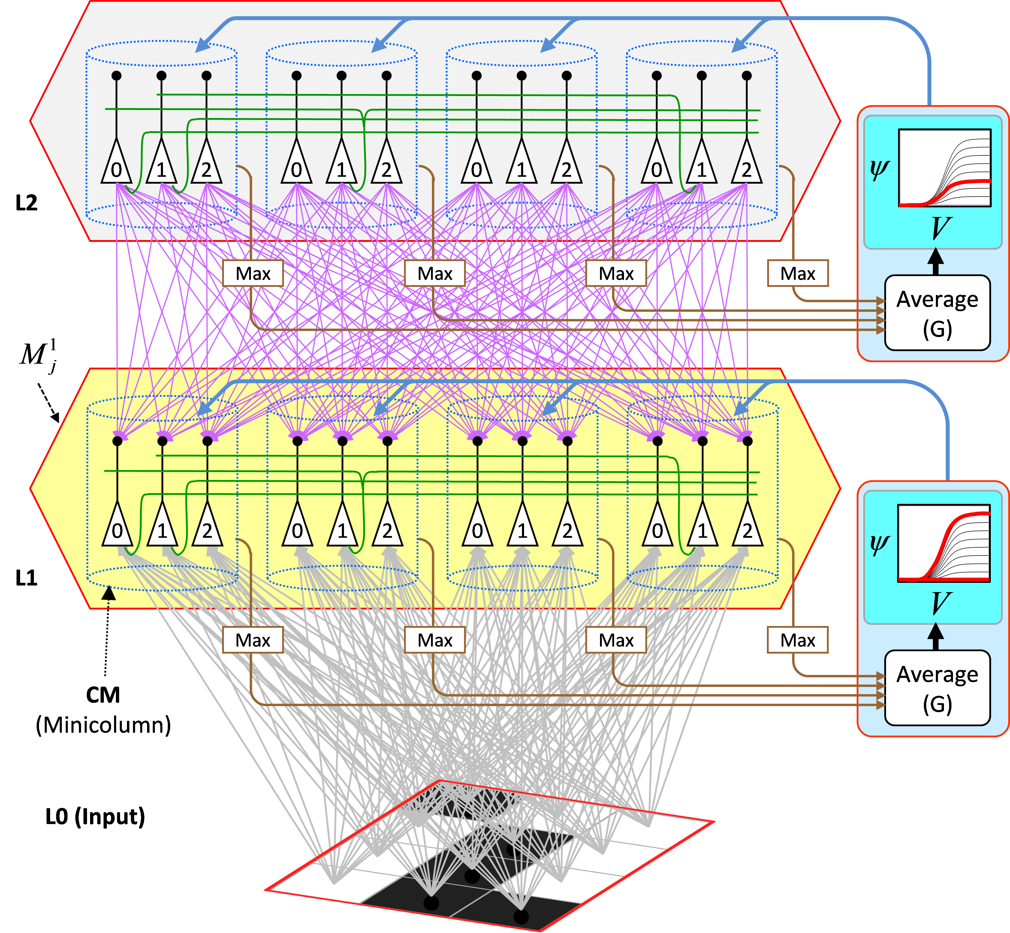
Figure 3: The core Sparsey circuit model. See text for description of its operaton.
The CSA can be summarized as consisting of three main operations. And see here for more detailed CSA explanation/demo.
- Each cell i sums and normalizes its U, H, and D inputs separately, resulting in three independent normalized (to [0,1]) measures of support (evidence) that it should become active, which are multiplied, yielding a total (dependent on H, U, and D inputs) local support measure, Vi, that cell i should activate.
- Then, the average of the maximal V value in each CM is computed, a value we call G. Because the mac's operation is constrained (during learning and recognition) so that only whole SDRs, i.e. sets of Q cells, one per CM, ever activate (or deactivate), G functions as a measure of the global familiarity of the total mac input. In the regime in which the number of stored SDR codes in the mac is sufficiently small (so that crosstalk remains sufficiently low), G in fact represents the similarity of the best-matching stored input (basis vector) to the current total input. As stated earlier the stored SDR codes represent particular spatiotemporal moments, as does the current total input.
- Finally, the global (i.e., mac-scale) measure G is used to modify the individual (local) Vi values of the mac's cells, on the basis of which the final winners (one per CM) will be chosen. To be more precise, the V values of all cells in a given CM are transformed via a function whose shape depends on G, resulting in relative (ψ), and then normalized to total (ρ), probabilities (within the CM) of winning. The final winners are chosen from the ρ distributions. The key to Sparsey's capabilities is that the compressivity of the V-to-ψ mapping varies inversely with G, or equivalently, varies directly with novelty (since familiarity is inverse novelty). When G=0 (max novelty), the V-to-ψ mapping collpases to a constant function, resulting in a uniform ρ distribution in each CM, and thus a completely random choice of winner. This corresponds to maximizing the expected Hamming distance of the newly selected mac code to all codes previoiusly stored in the mac. This code separation policy is appropriate: more novel inputs are assigned more distinct codes, which minimizes interference on future retrievals. This flattening of the distributions from which the winners are chosen can be viewed as increasing the amount of noise in the choice process. At the other end of the spectrum, when G=1 (max familiarity), the V-to-ψ mapping is made maximally expansive, resulting in a highly peaked ρ distribution in each CM, where the highest-ρ unit is the same unit that won on the prior instance of the current familiar input. This maximizes the likelihood of reactivating the entire code of that familiar input, i.e., code completion.
The net effect of the policy for modulating the shape of the V-to-ψ mapping based on G, is that as G (familiarity) increases the intersection of the winning code with the code of the best-matching stored input (hypothesis) increases and as G goes to zero, the expected intersection of the winning code with every stored code goes to chance. This is how Sparsey achieves mapping similar inputs (moments) to similar SDR codes, which we denote as the "SISC" property. See here for more detailed explanation and a demo of this policy.
We emphasize several unique aspects of Sparsey's CSA.
- To our knowledge, no other neural/cortical model implements the technique of using global (to a mesoscale unit, in our case, the mac) information to modulate local (to each individual cell) information, i.e., the cell's response function.
- This G-based modulation of the V-to-ψ mapping can be viewed as adding noise to the winner selection process, the magnitude of which is inversely proportional to the familiarity of the input, resulting in the SISC property. To our knowledge, this is a completely novel usage of noise in computational neuroscience.
- The astute reader will understand that the steps of the CSA algorithm imply a physical, neural realization which requires the principal cells, i.e., the units comprising the mac (which are intended as analogs of L2/3 pyramidals), to undergo two successive rounds of competition. In the first (in step 1 above), the cells of a CM compete on the basis of their V values, with only the cell with the max V becoming active in each CM. These max-V values are then summed and averaged, subserved by the brown arrows and boxes labeled "Max" in Figure 3 (this is a hard max). The pincipal cells are then reset whereupon the G-dependent noise is added to the mac. We hypothesize that this is subserved by one or more of the forebrain modulatory signals (e.g., NE, ACh) (cyan/blue arrows in Figure 3). This added noise effectively modulates the transfer functions of the principal cells, wherupon they compete again. Although we formalize the second competition as a draw from the ρ distribution (in each CM), i.e., soft max, the physical addition of the noise allows the soft max to be achieved via a hard max. The CSA's requirement of two rounds of competition is a strong and highly distinguishing model characteristic, an eminently falsifiable aspect of the theory. Our working hypothesis is that the two rounds of competition occur in the two half cycles of the local gamma oscillation.